-
Notifications
You must be signed in to change notification settings - Fork 339
Understanding data mining and prediction in one article
People always want to be able to predict the future, such as predicting tomorrow’s weather, predicting house price in a certain area, predicting next quarter’s sales, predicting customers’ buying preferences, and so on.

So, is there any way we can make predictions?
Let’s look at two examples.
In the evening, the pavement is somewhat moist after a light rain, a gentle west wind blows, and the sunset glow hangs in the sky.
Well, the weather will be nice tomorrow.
When we go to a fruit stand and pick out a watermelon with dark green skin, a curled stem and a hollow sound when tapped, we will look forward to enjoying this ripe melon.
From slightly wet road surface, gentle wind and sunset glow, we can predict based on our experience that the weather is nice tomorrow.
From dark green skin, curled stem, and hollow sound when tapped, we can predict based on our experience that the watermelon is ripe.
Both predictions are made based on our past experiences.
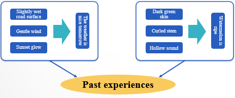
In mathematical language, the essence of prediction is to find a computable function that allows us to use observable information as input to calculate the expected prediction result as output.
In the example of picking watermelon, the skin colour, stem shape and tapping sound are the observable information, which are the input values; the quality of watermelon is the result we hope to predict. With such a function, we can make predictions.
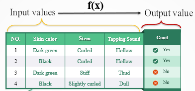
When we get a watermelon, observe its skin colour, stem shape and listen to the tapping sound, and then substitute the observed information into the function for calculation, we can get the prediction result.
We call this function a prediction model, or model for short.
So, how can we find this function?

Think about how to make a person have the ability to judge whether a melon is good or bad, what should you do?
For sure, it needs a lot of melons to practice.
Before cut the melon open, observe its characteristics, such as skin color and stem. Then cut it open to see whether it is good or not. Over time, you will be able to predict the quality of a melon based on its external characteristics.
Simply put, the more melons you use for practice, the more accurate your judgment will be in the future.
Every time you practice, you will obtain a set of input values, such as skin colour and stem of a melon, and an output value, such as good melon or bad melon.
After repeated practice, you will accumulate many sets of input and output values, which are historical data.
The function used for prediction is derived from historical data.
Let’s explain in professional terms.
The function used for prediction is also called a model.
The scientific name of the input values of a model is called feature variable, generally represented by x. There are often multiple feature variables, presented as a multi-column table, where each column is a feature variable. For example, in the watermelon picking example, skin colour, stem, etc are feature variables.
The scientific name of the output value of a model is called target variable, generally represented by y. For example, good melon or bad melon is target variable. The target variable can also be concatenated to the feature variable table, which is the general form of historical data.
The process of finding a model is modeling. When encountering new situations, using this model to calculate is prediction.
The whole set of technologies is called data mining. As the name suggests, it is to extract something valuable from the data, i.e., a model.
It should be noted that a model usually cannot achieve a 100% accuracy. Even the most experienced melon farmers cannot guarantee that they can pick good melon every time, and the weather forecast is not always accurate. Every model has an accuracy; as long as the accuracy is high enough, it still holds application value.
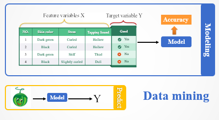
So, how do we use historical data to find models?
This brings us to the data mining algorithms.
For example, there is a set of data on house size and sale price. The house size is the feature variable x, and the price is the target variable y. Now we hope to use the house size to predict the price.
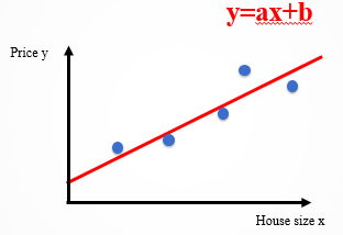
Through observation, we find that as the house size increases, the price generally rises in a linear trend. Therefore, we guess that there is a linear relationship between x and y.
Then, using the linear fitting method in mathematics to calculate a straight line y=ax+b can approximately describe the relationship of this set of x and y. That is, we can approximately calculate y from x, which is equivalent to finding the model.
This is a data mining algorithm called linear regression, which can be used for modeling when both x and y are numerical values.
Since the two sets of values in the watermelon picking example are not two sets of numerical values, the linear regression algorithm is not applicable. In this case, decision tree algorithm may be useful.
The principle of decision tree is completely different from that of linear regression. It can be seen as the set of if-then rules in a tree structure.
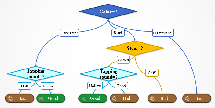
To be specific, each path from the root to the leaf of the decision tree constructs a rule. The characteristic of the internal nodes on the path corresponds to the condition of the rule, and the category of the leaf node corresponds to the conclusion of the rule.
Using historical data can gradually construct the full decision tree, which is modelling.
Even if it is a relationship between two sets of numerical values, it may not always be possible to use the linear regression algorithm to model.
For example, the figure below shows another set of data on house size and sales price.
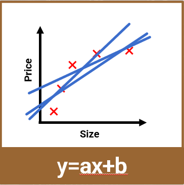
It can be seen from the figure that as the house size increases, the price also rises, but it is obviously not a rise in a linear trend. If we use the linear regression to calculate, we will find that no matter how we choose a straight line, the fitting effect is not very good.
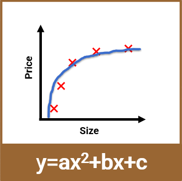
If we change the algorithm and add nonlinear factors, such as using a quadratic function, it fits very well.
Therefore, even for the same problem, different algorithms may be used.
Indeed, there are many algorithms for data mining, such as LASSO regression, logistic regression, support vector machine, decision tree and random forest.
Each algorithm has its own mathematical principles and a certain applicability. Different problems require different algorithms.
The currently popular AI LLM is essentially also a prediction model. It predicts the probability of the next word appearing in a sentence and selects the word with a higher probability to output. So, data mining is the predecessor of AI.
The algorithm used in LLM is called neural network, which is very complex and connected by nodes composed of layers of mathematical functions. It is large in scale and requires massive amounts of historical data for modeling.
These algorithms are the core of data mining and require a lot of mathematical knowledge to master. For example, if you want to understand regression algorithm, you have to understand the least squares method, gradient descent, multicollinearity, etc. Each algorithm has many parameters, and if you don’t understand the mathematical principles behind them, you won’t know how to proceed.
Moreover, understanding such mathematical knowledge is not enough. Historical data often cannot be used directly and needs to be preprocessed.
There are many preprocessing methods, such as handling missing values, data correction, cardinality reduction, normalization, discretization, data smoothing, and each method is not simple. For example, handling missing values involves more than ten approaches. All of these methods require a wealth of math knowledge to master.
Having built a model, there is also a need to test the model to check the error between the model and the real situation, which determines whether the model can be used for prediction.
Moreover, the modeling process isn’t a one-shot process. If the error is too large, that is, the accuracy is too low, then repeated adjustment is required.
Therefore, it often takes days or even weeks to build a usable model, and most of the time is spent on continuous adjustment and optimization, rather than simply applying the algorithm to the data.
Of course, all of this requires programming using a computer. If you are not a programmer, you should learn some programming knowledge.
Data mining and modeling is a highly complex job that can only be done by a small number of professionals, who are known as data scientists.

Obviously, it is not easy to train data scientists, so hiring good data scientists is expensive, making it a very promising profession. However, talented data scientists are few, which restricts the application scope of data mining technology.
Fortunately, the automatic data mining and modeling tools that have emerged in recent years break this constraint.
YModel, as an illustration, consolidates the mathematical knowledge required for modeling and the rich experience of top statisticians, allowing individuals who do not understand these advanced mathematical concepts to model with just one click.
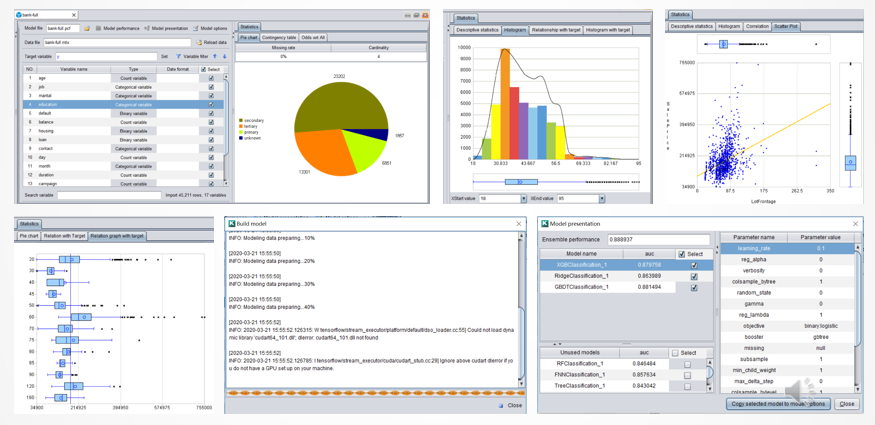
However, even if an automatic modeling tool is available, it is not as simple as just putting historical data into the tool and processing. To build a high-quality model, rich business knowledge is also required.
When modeling, it often needs to generate some new feature variables based on the original feature variable, and these new variables are called derived variables. With good derived variables, the model quality can be greatly improved.
For example, there is a feature variable which is the transaction date. If holidays are derived from it, the effect of making business forecasts will be much better than using the original date, because business activities are indeed closely related to holidays.
This information is relevant to business, and those with more business experience can work out more and more accurate derived variables, which does not require mathematical knowledge.
On the contrary, automatic modeling software is stronger in mathematical capabilities and can make up for the user’s deficiencies in math, but it has not and can not possess business knowledge and cannot perform tasks that rely on business experience for users.
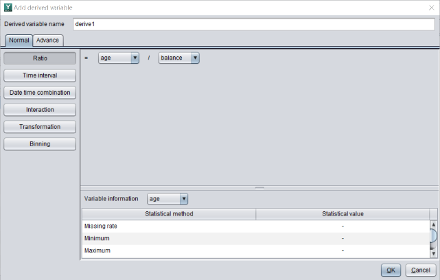
As a modeling tool, it is necessary to support users in adding derived variables. For example, YModel supports the addition of various derived variables such as ratio, interaction, binning, transformation, and date- and time-related variables.
The amount of historical data used for modeling should also be moderate. Unlike AI LLM, data mining does not require massive amounts of data; a few tens of thousands or hundreds of thousands of records are enough. Too much data will not significantly improve the model’s performance, but greatly increases the computation time and cost. Too little data, such as only a few or dozens of records, is not enough to find out pattern from the data.
From this point of view, data mining technology is highly operable. Most organizations can accumulate data of this scale as long as they have been operating for several years. Moreover, modeling does not require much computing power. For example, when using YModel to process data of this scale, a regular PC laptop is enough, with no need for a professional server cluster.
In addition, there is also a need to understand some knowledge related to model evaluation so as to know whether a model is good or not.
A basic indicator for evaluating a model is accuracy, which indicates the proportion of correct predictions among all prediction results.
Of course, we hope to make more accurate prediction, so we usually select a model with higher accuracy.
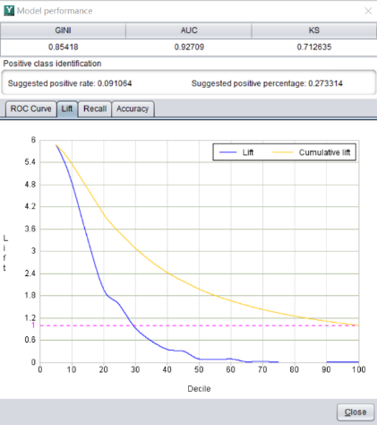
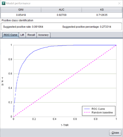
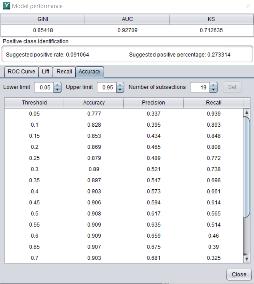
However, accuracy is not the only indicator to judge whether a model is good or bad. The following figures are the interface of YModel, which can automatically calculate many indicators, such as accuracy, recall ratio and AUC.
Different indicators have different meanings. Different business scenarios will focus on different indicators.
For example, a company wants to sell 50 products and has a list of potential customers.
If the company randomly selects customers to sell its products, it would probably need to contact several hundred customers to sell 50 products.
To improve efficiency, a model can be built to select target customers.
Those customers who ultimately purchase the product are called positive sample in data mining terms. Conversely, those who do not purchase the product are called negative sample.
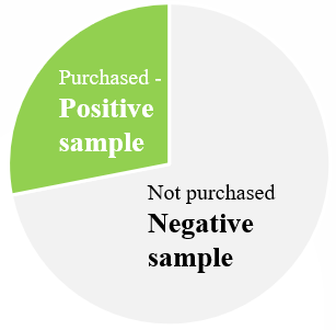
To improve the promotion efficiency, we will pay more attention to model’s accuracy in predicting positive samples, because we will only promote to the customers who are predicted to buy the product, and we will not care how high the accuracy is for the negative samples predicted by the model, because these customers will be discarded.
This indicator is called precision.
Precision represents the proportion of true positive samples among the samples predicted as positive. For example, if we predict 100 customers will buy the product and 60 of them actually do purchase it, then the precision is 60%.
For instance, the precision of model A is 67%, and the accuracy is 70%.

This figure indicates that among the customers predicted to make a purchase by Model A, 67% will actually make a purchase. Therefore, it is not difficult to deduce that if the company want to sell 50 products, it only needs to promote to 75 customers to achieve the goal, which greatly improves work efficiency.
Now let’s look at model B.

Although the accuracy has decreased, the precision has increased. Using Model B, promoting to just 60 customers can sell 50 products, reducing promotion cost.
Therefore, we should learn to use appropriate indicators to evaluate a model, rather than blindly pursuing accuracy.
Let’s look at another example. An airport wants to build a model to identify terrorists. Suppose there are five terrorists among one million people.
Since terrorists are an extremely small minority, if we use accuracy to evaluate the model, then as long as we identify all people as normal people, the accuracy of the model can reach as high as 99.999%, such as model A. However, it is obviously that such a model doesn’t make any sense. To effectively identify terrorists, it is necessary to build a model with a relatively high recall ratio.

Recall ratio represents the proportion of samples that are correctly predicted among the actual positive samples. For this example, it means how many of five terrorists can be caught.
For example, although the accuracy of model B is somewhat low, the recall ratio is very high. It can identify all terrorists. However, while it is possible to misidentify a few normal people as terrorists, it is much better than missing the terrorists. Therefore, such a model makes sense.

Different accuracy and recall ratios will generate completely different results.
The modeling tools like YModel have the functions of automatically calculating many indicators, such as accuracy, precision and recall ratio, making them very intuitive to use.

In addition to using numerical indicators to evaluate model performance, some graphics can be used to evaluate performance, such as lift curve.
Lift curve indicates how many times the performance will be improved after using a model, that is, the Lift.
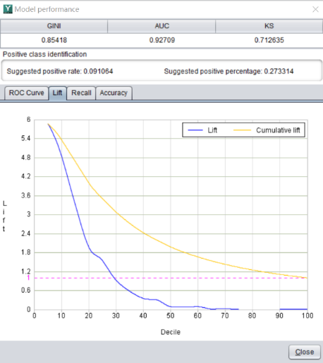
For example, in a telemarketing scenario for a certain product, there are one million potential customers, and the average purchase rate is 1.5%. This means that if one hundred customers are randomly selected, an average of 1.5 people will buy the product.
Now we use YModel to build a model to do a marketing prediction on the product, and the lift curve is shown as below.
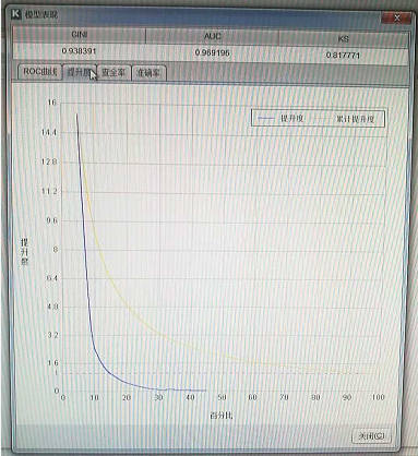
The model predicts that the lift for the top 5% of customers with the highest transaction probability is 14.4, which means that among the top 5% of customers, an average of 21.6 out of every 100 people will buy the product.
This result is far higher than 1.5 people out of 100 customers selected at random, which greatly improves marketing efficiency and reduces ineffective marketing activities.
In addition, the recall ratio graph is also very useful. For example, it can be used in risk claims scenarios.
The figure below is an analysis chart drawn using YModel for the built claim prediction model. It can be seen that among over 300,000 insurance policies, only 1,246 policies result in claims, and the positive sample rate is only 0.4%.
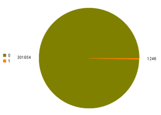
What the insurance company cares about is how to quickly identify high-risk customers from numerous policies so as to take measures to reduce claims losses. As can be seen from the recall ratio graph drawn with YModel, 75% of high-risk customers can be captured from the first 10% of the data.
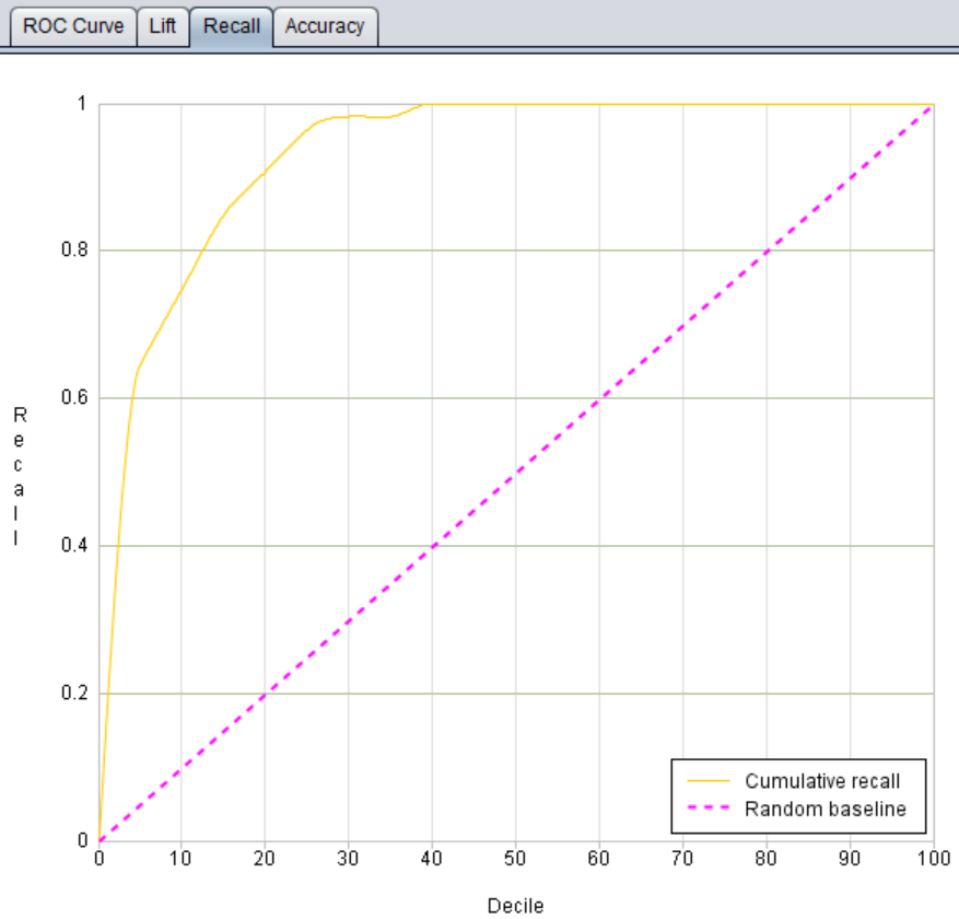
That is to say, among over 300,000 insurance policies, it only needs to screen 30,000 policies to capture 75% of high-risk customers, which greatly improves work efficiency.
In addition to model evaluation indicators, the stability of model should also be considered in practice.
For example, there are three models for the house price prediction data mentioned above.

The blue lines represent the predicted values fitted by the models, and the red dots represent the actual values.
Obviously, the model on the far right exhibits the highest accuracy.
But we should know that the goal of modeling is not to describe history, but to predict the future.
We prefer a model that performs well on unseen data. In professional terms, what we need is a model with better generalization ability.
Although the third model perfectly predicts historical data, it does not reflect the development trend of the data and performs poor in generalization ability. This situation is called overfitting.
The fitting effect of the first model is too poor, which is called underfitting.
Although the accuracy of the second model is not that high, it has good generalization ability and performs relatively stable in predicting data, making it a more ideal model.
Overfitting is a very common mistake, and special attention should be paid to avoid it during modeling. Statisticians have many ways to prevent overfitting. For example, YModel encapsulates a lot of statisticians’ experience and methods, allowing it to perform better than an ordinary programmer.
Data mining is a very useful AI technology, which can help people make various predictions and give us a stronger ability to gain insight into the future. As technology advances, automatic modeling technology has become increasingly mature. Using automatic modeling tools like YModel can significantly lower the threshold of data mining, allowing non-professionals to easily apply data mining technology and making it practical and feasible to predict the future.
SPL Resource: SPL Official Website | SPL Blog | Download esProc SPL | SPL Source Code