-
Notifications
You must be signed in to change notification settings - Fork 339
Python Is Not Built for Business People
Business people are used to performing data analysis with Excel. They also got used to the numerous frustrating or desperate situations when they are stuck on complicated calculations, repeated calculations and automated processing, and to add fuel to the flame, when system crash happens at this time but work hasn’t been saved.
Now they know that they don’t have to bear these situations anymore if they learn to use a programming language. But which programming language they should choose?
Python is your best choice! They are fed by computer programming companies and huge amounts of network information.
The language produces simple code in handling Excel troubles. It seems that it is the right one.
But the reality tells another story.
Daily analytical work mainly involves manipulating tabular data (the technical term is structured data), as shown below:

Except for the first row, each row of data is a record containing information about something or someone. The first row is headers that describe the attributes of record. All records have same attributes. A table is a set of these records.
Python provides DataFrame to handle tabular data. It works in this way.
DataFrame reads the above tabular data as this:

This looks like an Excel table. But the row numbers begin from 0.
A DataFrame is essentially a matrix (Can you recall your college linear algebra?). And Python doesn’t have the concept of record. All Python methods should be able to be suitable for doing matrix calculations.
Below are some simple operations.
The common and simple operation gets a subset meeting a specified condition. Based on the above data frame, for instance:

Task 1. Get records of employees in R&D department.
Python script:
| import pandas as pd data = pd.read_csv('Employees.csv') rd = data.loc[data['DEPT']=='R&D'] print(rd) |
Import Pandas Read in data Get records of employees in R&D department View data stored in rd |
Execution result:

The script is simple and the result is correct. But there are two other things you need to know:
1. The key function the script uses is loc, which is the abbreviation of location. It isn’t a filter function. Python achieves the filtering indirectly by using it to locate the indexes of rows meeting the specified condition. data[‘DEPT’]==’R&D’ within the function generates a Series consisting of Boolean values.
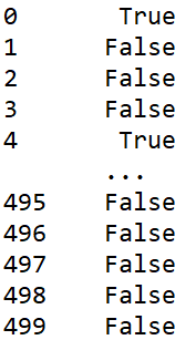
Get indexes whose corresponding rows meet the specified condition and record them as True; otherwise record them as False.
Then loc gets rows from data according to indexes recorded as True to generate a new DataFrame. The operations are basically extracting specified rows from a matrix. It’s a roundabout way to do filtering.
2. There are other methods to filter a DataFrame, such as query(…). All of them involve locating indexes of rows or columns in a matrix and then retrieving data by these indexes. Their syntax is generally in the form of matrix.loc[row_indexer,col_indexer].
It seems that the most basic filtering in Python is not too hard to understand. The following calculations are concerned with the filtering result, the subsets.
Task 2: Give a salary increase of 5% to employees in R&D department.
The intuitive solution is to select employees in R&D department and modify their salaries.
The corresponding script is like this:
| import pandas as pd data = pd.read_csv('Employees.csv') rd = data.loc[data['DEPT']=='R&D'] rd['SALARY']=rd['SALARY']*1.05 print(data) |
Import Pandas Read in data Get records of employees in R&D department Modify SALARY values |
Execution result:
SettingWithCopyWarning:
A value is trying to be set on a copy of a slice from a DataFrame.
Try using .loc[row_indexer,col_indexer] = value instead
See the caveats in the documentation: http://pandas.pydata.org/pandas-docs/stable/user_guide/indexing.html#returning-a-view-versus-a-copy
rd['SALARY']=rd['SALARY']*1.05

A warning was triggered and modification failed too.
That’s because rd = data.loc[data['DEPT']=='R&D'] is a submatrix. We modified the submatrix, instead of the original matrix, because rd['SALARY']=rd['SALARY']*1.05 generated a new matrix by updating SARLARY values.
It’s hard to express and understand.
The correct script is as follows:
| import pandas as pd data = pd.read_csv('Employees.csv') rd_salary = data.loc[data['DEPT']=='R&D','SALARY'] data.loc[data['DEPT']=='R&D','SALARY'] = rd_salary*1.05 print(data) |
Get salaries of employees in R&D department Calculate the new salaries for employees in R&D department and perform update |
Execution result:

We got the correct result this time. So you shouldn’t get the subset to modify. Instead you need to first locate the indexes of the to-be-modified members from the original matrix, which is loc[row_indexer=data['DEPT']=='R&D',column_indexer='SALARY']), get the target data according to row and column indexers, and assign new values to the matrix. To get a 5% salary raise, you also need to get the to-be-modified SALARY values using the statement rd_salary = data.loc[data['DEPT']=='R&D','SALARY'] before the assignment. The repeated filtering results in inefficient and very roundabout code.
Task 3: Find records of employees in R&D department who come from the New York state.
It is simpler. We just need to get the two subsets and calculate their intersection. Below is Python’s solution:
| import pandas as pd data = pd.read_csv('Employees.csv') rd = data[data['DEPT']=='R&D'] ny = data[data['STATE']=='New York'] isect_idx = rd.index.intersection(ny.index) rd_isect_ny = data.loc[isect_idx] print(rd_isect_ny) |
Get records of employees in R&D department Get records of employees who come from New York state Get intersection of the indexes of rd and ny Get records according to intersection of indexes |
Execution result:

Getting intersection of sets is a basic operation many programming languages support. Python offers intersection function to do it. The point is that a DataFrame is fundamentally a matrix but that getting intersection of two matrices makes no sense. So Python doesn’t provide a special method to calculate intersection of matrices. In order to implement the intersection operation on sets represented in the form of DataFrame, the language gets intersection of the matrices’ indexes and then locates and intercepts data according to it. The route is roundabout and tricky.
As one of the most basic operations, Python filtering is already so hard to understand. You can imagine how unintelligible and tortuous of the methods for implementing more complicated operations.
Grouping is one of them.
Grouping is common in daily analysis work. Python has abundant relevant functions to be able to handle most of the grouping tasks. But they are not easy to understand and use.
Grouping is to divide a set into a number of smaller sets according to a specified rule. The grouping result is a set of sets and you can perform one more operations on the subsets, as the following picture shows:
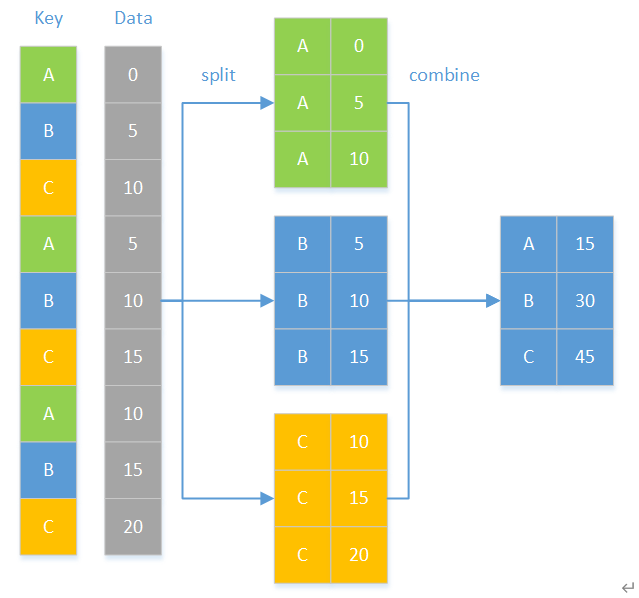
Grouping and then aggregation is the most common grouping operation.
Task 4: Count the employees in each department.
The Python script:
| import pandas as pd data = pd.read_csv('Employees.csv') group = data.groupby("DEPT") dept_num = group.count() print(dept_num) |
Group records by department Count employees in each department |
Execution result:

The result is weird. What we need is one column that records the number of employees in each department (group). But there are many same columns as if each column was counted.
Python fixes the error by replacing count function with size function:
| import pandas as pd data = pd.read_csv('Employees.csv') group = data.groupby("DEPT") dept_num = group.size() print(dept_num) |
Group records by department Count employees in each department |
Execution result:
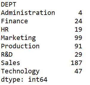
The result is improved. But it seems that there is still something wrong with it.
Yes, this is not a two-dimensional DataFrame anymore. It is a one-dimensional Series.
We get the first result because count function performs count on every column. The size function gets it right because it measures the length of each group. But it’s more natural for us to use count instead of size (we need to have more information to know the method) to get the total number.
A grouping result, as we said above, should be a set of sets, but what about the result of grouping a Python DataFrame? Let’s print the result of data.groupby(“DEPT”).
| import pandas as pd data = pd.read_csv('Employees.csv') group = data.groupby("DEPT") print(group) |
Group records by department |
Execution result:
<pandas.core.groupby.generic.DataFrameGroupBy object at 0x000001ADBC9CE0F0>
What the hell is this?
Probably it is a shock when you first see this. It can be a nightmare for a non-professional programmer.
A search on the internet tells us that it is an iterable, where each group consists of the group index and a DataFrame after we iterate through it. There are a number of methods, such as list(group), to view the details, as shown below:

It is basically a set of sets if we also regard a matrix as a set. But we can’t get a member directly from a matrix as we do from an ordinary set, as group[0] does. We have to cram a number of rules in for performing operations on such an object if we can’t understand them.
You may be completely confused now. “This sounds like quite a bit of gobbledygook!” You may think to yourself. But never mind – this is normal for an ordinary business person.
Now let’s move further on to see a more complicated scenario – operations on the subset after data grouping.
At times we are not concerned with the aggregates but the status of the subsets, such as sorting by a certain column on each of them.
Task 5: Sort records of employees in each department according to the hire date in ascending order.
Analysis: Group records and then sort each subset by hire date.
The Python script:
| import pandas as pd employee = pd.read_csv("Employees.csv") employee['HIREDATE']=pd.to_datetime(employee['HIREDATE']) employee_new =employee.groupby('DEPT',as_index=False).apply(lambda x:x.sort_values('HIREDATE')).reset_index(drop=True) print(employee_new) |
Modify hire date format Group records by DEPT, sort each group by HIREDATE, and reset the index |
Execution result:
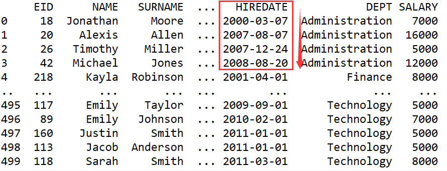
The result is correct. Now let’s look at the core statement (employee.groupby('DEPT',as_index=False).apply(lambda x:x.sort_values('HIREDATE'))) in the script. Below is the syntax of the statement:
df.groupby(c).apply(lambda x:f(x))
df: DataFrame
groupby: Grouping function
c: The column used as grouping basis
But the cooperation of apply function and lambda is well beyond most of the non-programmers. One needs to be familiar with the principles of functional language to understand it (I won't go into trouble to explain it here. You can google it by yourself.).
A more complicated alternative is using for loop to sort each subset separately and then concatenate the sorting results.
| import pandas as pd employee = pd.read_csv("Employees.csv") employee['HIREDATE']=pd.to_datetime(employee['HIREDATE']) dept_g = employee.groupby('DEPT',as_index=False) dept_list = [] for index,group in dept_g: group = group.sort_values('HIREDATE') dept_list.append(group) employee_new = pd.concat(dept_list,ignore_index=True) print(employee_new) |
Modify hire date format Group records by DEPT Initiate a list for loop Sort each group separately Put sorting results to the above list Concatenate the sorting results |
The result is same but the script is much more complicated and inefficient.
Python gives different data types and devises different methods for handling essentially same data but of different formats. Users can’t apply an effective method to all similar data in nature. This leaves users really confused and annoyed.
In short, Python is hard to understand and learn because it is professionally-oriented. Here are three aspects for illustrating this:
1. The essence of DataFrame is matrix.
All operations need to be implemented with methods that can be applied in matrices. So many methods are roundabout.
2. Complicated data types with inconsistent rules
Python has Series, DataFrame, GroupBy object and many other data types, but designs different computing rules for them. For instance, you can use query function to filter a DataFrame but not a Series. Compared with the other two, the GroupBy object is a disparate type and has more complicated rules.
3. Easy to imitate but hard to understand
As Python has too many data types and according computing rules, learners need to memorize more but have more difficulty to use it flexibly. One strange thing is that it takes longer to search for a Python script on internet for a computing task than to get it done with Excel.
That Python is simple is just a false impression. Even if you enroll in a training session, probably you can just learn how to copy a solution but can’t truly master it.
If we had a tool intended for business people.
And there is one.
esProc SPL is a programming language specialized in handling structured data. SPL (Structured Process Language) provides plentiful basic computing methods conforming to our intuitive, natural way of thinking.
1. A table sequence is a set of records.
SPL uses Excel-like table sequence to display structured data.
2. Concise data types with consistent rules
Generally SPL structured computations involve only two data types – set and record – based on consistent rules.
3. Easy to use and learn
You only need to know the two data types and learn the basic computing rules to be able to handle both simple and more complicated tasks. By combining and coordinating the basic and simple rules, you can handle any complex scenarios. With SPL you may write a not graceful script but you are sure to produce one quickly. You don’t need to search for a code solution as you do with Python.
Now let’s take a look at SPL’s easy, intuitive and smooth coding style.
esProc SPL uses table sequence to store two-dimensional structured data. The layout is same as an Excel worksheet, as shown below:

In this table sequence, each row, except for the first row that contains column headers, is a record. A table sequence is a set of records. It is intuitive compared with Python DataFrame.
Instead of locating members in a matrix, SPL selects eligible records directly.
Task 1: Get records of employees in R&D department.
| A | B | |
|---|---|---|
| 1 | =file("Employees.csv").import@tc() | / Import data |
| 2 | =A1.select(DEPT=="R&D") | / Perform filtering |
A2’s result:

The SPL result is a subset of the original data set, which is easy to understand.
Let’s move on to see how SPL works to modify data in subsets and to get intersection of subsets.
1. Modify data in the subset
Task 2: Give a salary increase of 5% to employees in R&D department.
| A | B | |
|---|---|---|
| 1 | =file("Employees.csv").import@tc() | / Import data |
| 2 | =A1.select(DEPT=="R&D") | / Get eligible data |
| 3 | =A2.run(SALARY=SALARY*1.05) | / Modify SALARY values |
| 4 | =A1 | /View result |
A4’s result:

SPL first finds eligible records and then modifies the salary values. The process is more in line with intuitive human thinking.
2. Get intersection of subsets
Task 3: Find records of employees in R&D department who come from the New York state
| A | B | |
|---|---|---|
| 1 | =file("Employees.csv").import@tc() | / Import data |
| 2 | =A1.select(DEPT=="R&D") | / Get records of employees in R&D department |
| 3 | =A1.select(STATE=="New York") | / Get records of employees who come from the New York state |
| 4 | =A2^A3 | / Get their intersection |
A4’s result:

SPL intersection operation is a true set operation because it gets the intersection directly over two sets. So a simple operator “^” is enough to express the operation. Unlike Python’s extremely roundabout method, SPL intersection syntax is easy to write and understand. Other set operations, including union, difference, OR, etc., also use operators to express. This is simple and convenient.
The result of a SPL grouping operation is a set of sets, which is clear and intuitive.
Let’s first look at grouping & aggregation.
Task 4: Find the number of employees in each department.
| A | B | |
|---|---|---|
| 1 | =file("Employees.csv").import@tc() | |
| 2 | =A1.groups(DEPT;count(~):cnt) | /Grouping |
A2’s result:
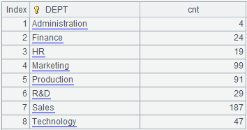
The result is also a table sequence. So you can use same methods to handle it. Python, however, gets a result of one-dimensional Series, which is a different type.
Here’s SPL’s grouping result:
| A | B | |
|---|---|---|
| 1 | =file("Employees.csv").import@tc() | |
| 2 | =A1.group(DEPT) | /Grouping |
A2’s result:
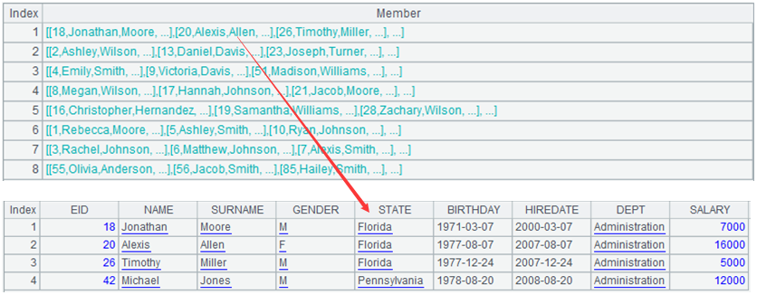
It is a set of table sequences. Each subset is a table sequence consisting of records of employees in a same department. The picture also shows the table sequence made up of members of the first group (the Administration department).
The result conforms to the natural, intuitive logic and easy to view. It’s also convenient to perform other operations on the subsets.
Since a SPL grouping result is a set of sets, so you can directly perform any operations on a subset.
Task 5: Sort records of employees in each department according to the hire date in ascending order.
| A | B | |
|---|---|---|
| 1 | =file("Employees.csv").import@tc() | |
| 2 | =A1.group(DEPT) | /Grouping |
| 3 | =A2.conj(~.sort(HIREDATE)) | /Sort each subset and concatenate them |
A3’s result:

As the grouping result is also a set, you can use set-related methods to further handle it. The language implements grouping, sorting and concatenation smoothly with a 3-line script. The script is easy to write and understand and efficient. No more cramming up and the unintelligible apply()+lambda duo.
1. Python structured computations are fundamentally the matrix computations. You cannot bypass handling matrix when implementing an operation even as simple as a set operation. esProc SPL is based on sets of records. So it can implement set operations in a simple and convenient way.
2. Python has complicated data types and changeable computing rules. It’s too difficult to learn and understand. Users highly depend on rote learning to write code. Usually they can learn to find out how to do a task but can’t understand why they should use the method. It’s almost impossible for them to handle similarly various scenarios flexibly. esProc SPL has simple and concise data types and offers more uniform and universal computing rules. So users are able to use the basic rules to handle complicated computing tasks in an adaptable and flexible way.
3. To learn SPL, please visit SPL Programming.
SPL Resource: SPL Official Website | SPL Blog | Download esProc SPL | SPL Source Code