tech_tonescale
In this page we will discuss methods for compressing a range of intensity values into a reduced range. For this we will need ... math.
"AAAAAAAAAAAAAAAAAAAAAAAAAAAAAAAHHHHHHHHHHHHHHHHHHHHHHHHHHHHHHHHHHHHHHHHH!!!"
--Angry Reader
Don't be scared Angry Reader! It's not going to be complicated or scary. I'll do my best to dumb it down to be as accessible as possible.
"I'm not dumb. F@!* you."
--Angry Reader
Before we get into more detail about tonescale approaches, let's do a little refresher on math and functions.
We'll use a plotting tool called Desmos here for visualizing some simple graphs.
A function is a mapping of an input value to an output value. If we graph a function in a 2 dimensional coordinate system, we can visualize the relationship between the two values. We take some input value on the x-axis, apply some process of change to it, and we get an output value on the y axis.
If you've used the ColorLookup tool in Nuke this is the same thing, but we are "creating our own function" by adjusting the curve.

Let's look at a simple example. Here is the graph of a function. f(x) = x.
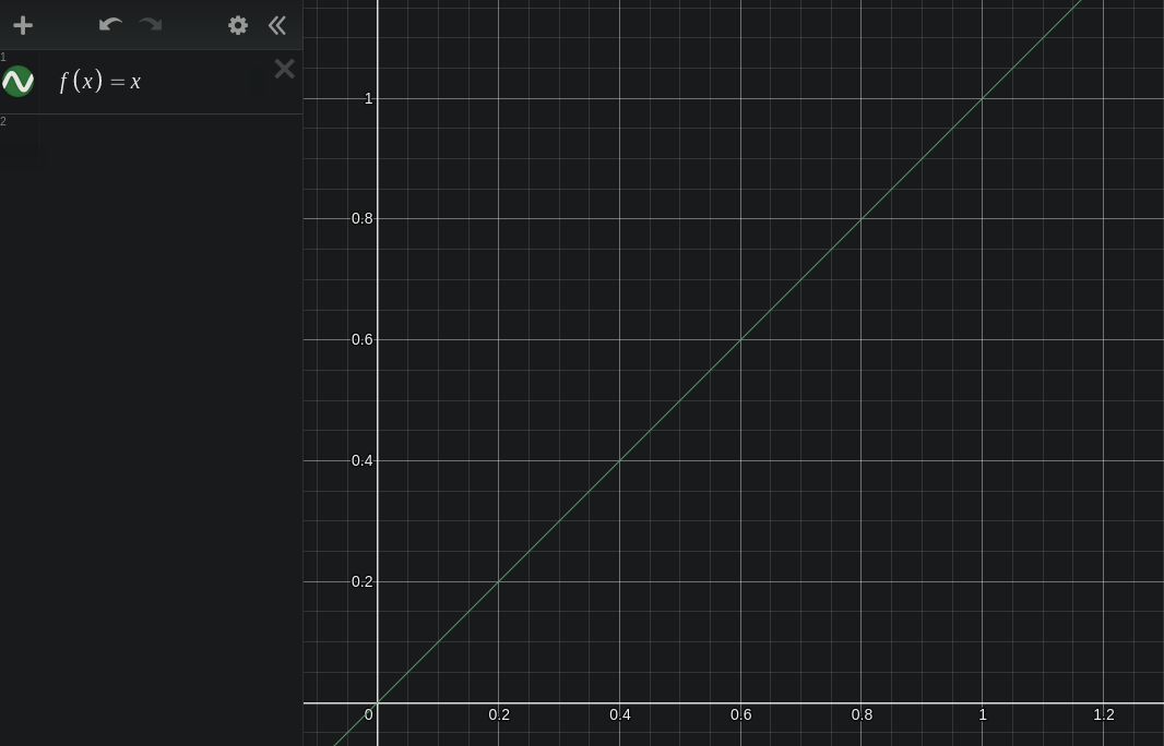
We have a function of the variable x, which is equal to x. So the input is x, and the output is unchanged. The resulting graph is a linearly increasing line with a slope of 1. Input values on the x axis are equal to output values on the y axis. Pretty boring!
Let's add some sort of change to the variable x so that the "process of change" is actually doing something. Here is a plot of y = m * x, where the constant m = 0.5. Here x is a variable because it is continuously varying, and m is a constant because it is set to a value that does not change.
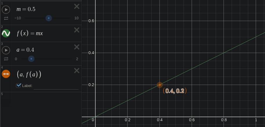
Our line is still straight, but it is tilted down a bit. The slope of the line is now 0.5 instead of 1.0.
Above I'm also running another constant a through the function by typing f(a). This runs the value a through the function and returns the result. When a = 0.4, the output of the function is 0.5 * 0.4 = 0.2.
So now we know how a function maps an input value to an output value. Let's move on to finding an interesting "process of change" that could work for a Tonescale.
So what is a tonescale exactly? Breaking apart the word you might reasonably conclude that it is a process of scaling or compressing tonality. This is essentially it, but as usual, the devil is in the details.
The goal is to compress scene-referred image data into the reduced range of a display-referred image. Put another way, the goal is to take scene light energy and transform it into display light energy.
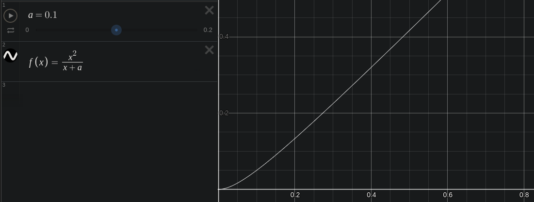
One very well-known tonemapping method is the "Reinhard" function: y = x / (x + 1), where x is the input pixel value, and y is the output pixel value.

This is a hyperbolic function.
"This looks awful. I want an S-Shaped tonemapping function! You're stupid!"
--Angry Reader
Well what if I told you dear angry reader, that this curve is actually s-shaped? Let's look again, but change the scale of the X-Axis so that it is on a logarithmic scale instead of a linear scale.
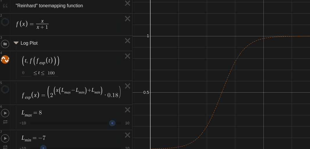
Viewed on this semi-log plot a hyperbola looks like an "s-shaped" sigmoid function!
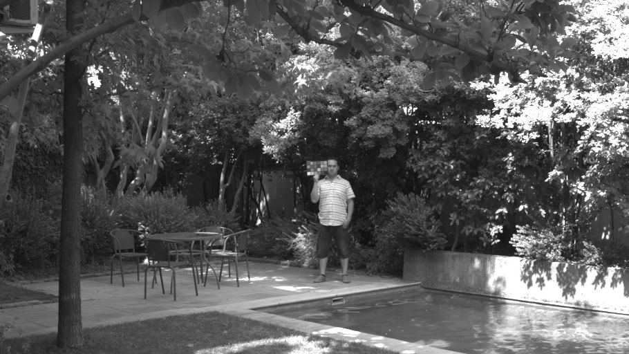
"This looks like garbage! Look at those clipped highlights!! Where is the color?! This tonemapping sucks a donkey di--"
--Angry Reader
Calm yourself angry reader! This is just the scene-linear image dumped directly to the display! We could think of this image as the light intensity of the scene mapped directly to the light intensity of the display. Beyond a certain point, the display can no longer get any brighter, and this is where the highlights "clip".
Here is the same image with the simple hyperbolic tonemap applied.

The midtones and shadows look pretty similar, but the highlights have a soft "rolloff" as they get brighter. This compression in the highlights allows us to preserve tonality in the image.
Scale
Let's see what other variables we can add. If we a scale for the input x and a scale for the output y this could be useful. This would allow us to control exposure of both input and output values.
y = s_y * (x / (x + s_x))
Now we can adjust the constants s_x to adjust the scene-linear input exposure, and s_y to adjust the display-linear output.
Power
The hyperbolic compression function converts scene-referred to display-referred. In display-referred it will be useful to have a power function (also known as a "gamma" adjustment). A scene-linear exposure adjustment is functionally similar to a "gamma" adjustment in display-linear. If we "gamma up" in display-linear, it is similar to adjusting exposure in a scene-linear. A "gamma" adjustment will also be useful for modeling surround compensation for different viewing environments.
Here is our test image with the above tonescale curve.

It has a bit more contrast than the pure hyperbolic curve: there is compression in the shadows and in the highlights now.
- If we want a bit more shadow compression we could boost the
pvariable - If we want to adjust overall exposure, we could adjust the scene-linear scale
sx - If we want to adjust where our scene-linear input clips in display-linear, we can adjust the display-linear output scale
sy. - If we want to increase "contrast", we could boost
pand also boostsx, to "gamma down, gain up".
So above we have the different parameters or "axes of movement" for our tonescale. We would want to carefully set each of these to achieve a good rendering for a specific viewing condition.
Viewing Condition
A term encompassing a viewing environment: The display and its luminance characteristics, the surround illumination conditions, and the viewer.
I did a lot of poking around comparing different approaches in the realm of sigmoid functions. Amongst my many dead ends and failed experiments, I did come across a super interesting bit of research describing the behavior of cone cells adapting to changes in stimulus with the Michaelis-Menten equation and its derivations like the Hill-Langmuir equation and the Naka-Rushton equation. These functions are usually used to model biological phenomena like enzyme kinetics, but the shape of the function fits very well the problem at hand. There are many scientific studies linking these. Of course this equation does not claim to model any of the higher order brightness processing that happens in the human visual system after the cone cells.
There is one piece missing still: flare/glare compensation.
Display devices are not perfect. We watch them in a living room with white walls. Reflections of the white wall behind us appear on the screen over the image and cause glare.
Display devices usually can not represent a pure black color. Especially LCD devices have a high minimum illumination or flare level. These factors contribute to reducing the apparent contrast of the image.
To compensate, we need to increase contrast in the image to compensate.
"I know how to increase contrast, we'll just boost the p and sx variables in the above equation!" -- Angry Reader
Actually for this type of compensation, we need a different shape of function which will compress much more the values near 0. We will use a parabolic compression function.

Here is our test image with a flare compensation of 0.01. The shadows are a bit more crunched down.
Nuke Script
Here is a nuke script with the tonescale functions above.
Full credit for the above math goes to Daniele Siragusano, who posted a variation of the above functions on acescentral. His post indirectly taught me everything I'm presenting here.
It is common practice for digital cinema cameras to subtract a small value from their images so that the average pixel value in deep shadows is 0. Because of digital sensor noise, this results in scene-linear values in deep shadow grain going negative.
Let's take a look at an example, another testimage from the excellent CML.

This image is shown here without any view transform. Let's take a look at the shadow area under the fire-extinguisher.
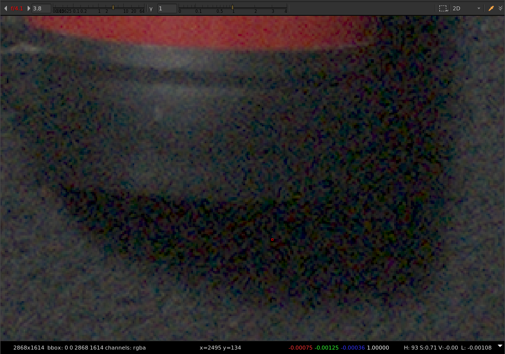
Sampling the value of a dark pixel in shadow grain we can see it is a small negative value.
Arri Classic LogC to Video Rec.709

Here is the same area rendered through an Arri display transform. Note that this negative pixel has been remapped to a relatively large positive value!
ACES Rec.709 Output Transform
 The ACES system does the opposite of the Arri transform. It maps a positive number to zero through the display transform. In the case of SDR, 0.002 in scene-linear is mapped to 0 in display linear and clipped. Because of this method we are losing tonality in deep shadows.
OpenDRT Rec.1886

Here is the same image using the tonescale method described on this page, rendered through OpenDRT.
This method maps scene-linear 0 to display-linear 0. Mapping black this way, and adjusting flare compensation with a parabolic compression function does a better job at preserving tonality in deep shadows, and reducing artifacts from hyper-saturated shadow grain.
This method is also a much better starting point for HDR display transforms, in which shadow level becomes much more important than in SDR.

Another important consideration in designing a tonescale for a display transform is how we map middle grey. Where we place middle grey in the range of display output luminance, determines the exposure of the image, and how the midtones and shadows are distributed, and how much headroom is left for highlights.
For SDR, the common standard is to map an input scene-linear middle gray value of 0.18 to a display-linear output value of 0.1. There is an interesting post on acescentral from Josh Pines on this topic which is worth a read.
How this mapping changes in HDR is an interesting (and emerging) topic, which I'll talk a bit more about on the HDR page.
"I've been a colorist for 75 years and I always work on log encoded imagery. All of this hyperbola mumbo-jumbo sounds like horse-shit to me."
--Angry Reader
Log is not going anywhere. It remains a very useful representation for scene light intensity data. There is a long history of colorists grading directly from log footage. It is an intuitive encoding to manipulate tonality. And probably the most common DI workflow today is to grade camera log footage with a CDL prior to some display transform.
The reason we use a hyperbolic compression function in the linear domain is that it reduces complexity. Generally speaking, applying a sigmoid in a log domain involves more transformations to the data and a big overhead in system complexity. The end result can be the same, but the system is more simple working directly in the linear domain. I believe that avoiding unecessary complexity is a good design goal.
Here's an example with the only other open domain display transform that I am aware of: The ACES system. The ACES Output Transform is very complex. I should know, I implemented it in blinkscript and nodes for Nuke. I would say it is so complex that it is effectively a black box for anyone but the most stubborn of technical geniuses (joking).
The tonescale of the ACES SDR Output Transform first transforms input scene-linear data into a pure Log base 10 encoding. Then a multi-segment cubic bezier spline is calculated for a min, mid, and max value. This forms the sigmoid curve. The data is then transformed back into linear, the tonescale applied. The SDR transforms use two stages of these curves. The CTL code for only the tonescale, is around 1,000 lines of code. And it will barely run on a GPU because of the splines.
The tonescale described here is a simple formula and could be represented as a single line of rendering code.
"Your single line of rendering code is crap! It doesn't map 0.18 to exactly 0.10. I need to know where my image values fall, otherwise the world will descend into chaos and madness!!"
--Angry Reader
I once thought like you Angry Reader. But then I did a great deal of experimentation and realized that exact mappings are not really that important in the grand scheme of things. See that image of the macbeth chart above? That's the Arri LogC2Video display transform. It maps input 0.18 to around 0.109, but it's not exact, and that is okay. More important is creating a good model for image appearance using the "axes of movement" we have above. This is even more important for HDR.
Next...