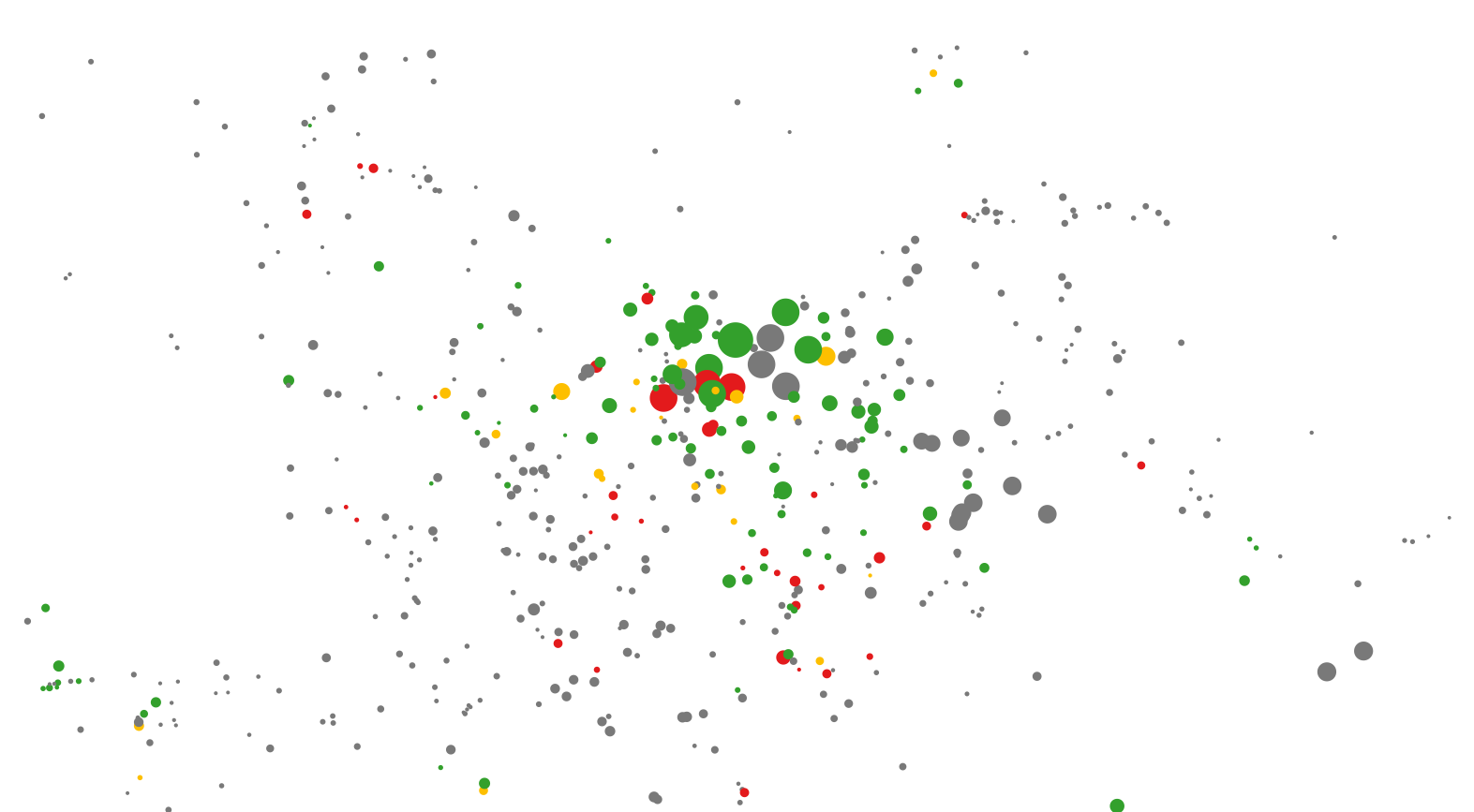
The purpose of this exercise is to use two sources of data with different contextual focuses in order to produce a visualisation that portrays the accessibility of popular places. The two datasets that will be used are Wheelmap and Foursquare Venues.
Wheelmap is a service developed by Sozialhelden in Berlin which aims at allowing users to view and edit whether a place is accessible to wheelchair users. The base data used are POI features from OSM, with the accessibilty information being stored agains the POI in the OSM dataset. The possible values for this accessibility are "yes", "limited", "no" and "unknown".
The foursquare data is the same as used in other examples, in particular the foursquare_venues_helsinki dataset.
Step 1: add the wheelmap_helsink csv file to QGIS as a layer. To do this, click on the "Add delimited text layer" from the "Manage Layers Toolbar" (the comma). Select the csv file and the rest of the information should be entered automatically. If not, the File format should be CSV, Geometry definition set to "Point coordinates", X field set to "lon" and the Y field set to "lat". click OK to add the file as a layer. If asked, select "WGS 84" as the CRS.
Step 2: Add the foursquare_venues_helsinki csv file as in step 1, but make sure that you set X field to "lng" and Y field to "lat".
Step 3: Now we need to join the foursquare data with the wheelmap data. To do this, right click on the wheelmap layer and select Properties. Under the Joins tab, click the small green + sign towards the bottom of the window. From here, set Join layer to be the foursquare layer, and then Join field and Target field to be name. This tells QGIS to match any record from the foursquare layer to one of the wheelmap layer with the same name. Obviously this is not perfect (POIs like McDonalds will appear in both datasets multiple times) but for now, it gives a good example. Finally, click on OK.
Step 4: Now that the layers are joined, if you view the attribute table for the wheelmap layer, you will see that many of the features will also contain foursquare information. At this point we want to create a visualisation that shows the accessibility of each venue as well as its popularity. For this example, we will use the colour visual variable to represent the accessibility and the size to show the popularity. Right click on the wheelmap layer again and select Properties followed by Style.
Step 6: As we will be using more than one variable to change the appearance of the features, we need to use the Rule-based style option from the drop down box at the top of the window. To create the visualisation you will need to create four rules. To create a rule, click on the green + button towards the bottom of the window. This will open up the rule properties dialogue. For the first rule, type Unknown for the label. This is what will be displayed in the legend. The actual rule generation is made by clicking on the ... button next to the Filter text box. In the Expression string builder, first click on the arrow next to Fields and Values to show all the fields that are available for the feature. Double-click on accessible to add the field to the text area (you can actually just type in the field name surrounded by double quotation marks). Type in the text area to make the text "accessible" = 'unknown'. This tells the rule to only be applied to feature that have a accessibility value of unknown.
Step 6: Now, we also need to make sure that this is only applied to features that have been matched with foursquare items. To do that, type in the same box AND "foursquare_venues_helsinki_id" IS NOT NULL. This tells the rule to only include features that actually have an id obtained from the foursquare dataset. The text area should now contain the text "accessible" = 'unknown' AND "foursquare_venues_helsinki_id" IS NOT NULL. Click on OK.
Step 7: Now we need to create the appearance of the point feature. For the "Unknown" category it is recommended to use a grey colout for the point. This is done by clicking on the Color box and selecting a grey colour. To change the size of the point based on its popularity, we click on the button next to the box with a label Size. This button should be an image that looks like two small rectangles on top of each other and a dark triangle to the side. Clicking on it opens up a menu where you want to select Size Assistant. This opens up another window where you can tell the system to make the size of the shape dependent on another value.
Step 8: In the size assistant, select foursquare_venues_helsinki_checkincount for the Field area. Set Scale method to be Flannery (you can play around with the different options) and leave the other values as they are (this should be 1 - 10 for the size, and 1 - ~86779 for the values). Click on OK, followed by OK in the Rule properties window.
Step 9: You have now created the rule for the "Unknown" category. To create the others, repeat steps 6-9 three more times, but rather than entering 'unknown' in the "accessible" = 'unknown' rule string and selecting a grey colour, enter 'no' and a red colour, 'limited' and a yellow colour, and 'yes' and a green colour.
Step 10: Finally click on OK and you should see a series of circles where the colour identifies accessibilty and the size is the popularity.
And a little extra: For those of you wanting to play around with accessing additional services, it is possible within QGIS to display a layer which is generated from GeoJSON (amongst others) directly from the web. For now, one thing that can be done is to show in QGIS an accessible route between two locations. For the CAP4Access project at Heidelberg University there has been an extension to the OpenRouteService not only to provide routes that are accessible, but also to deliver these routes in a GeoJSON format. First, find out the coordinates of the start and end locations. To find out these values, use the Identify features tool (the arrow with an i by it) and select the point you want the information for. The latitude and longitude values are displayed in the Identify Results pane by lat and lon (you may need to expand the pane to see them).
To add an accessible route to the map, add a new Vector layer but rather than selecting a file, choose the Protocol method and make sure that Type is set to "GeoJSON" Then in the URI box, enter http://cap4navi.geog.uni-heidelberg.de/NavigationService-1.5/CreateRoute?startLng=xxx&startLat=xxx&endLng=xxx&endLat=xxx&type=wheelchair, replacing the lat and lng values for those of two items from the wheelmap layer. Click on OK and the route will be displayed on the map (there may be a slight pause while it gets the data).
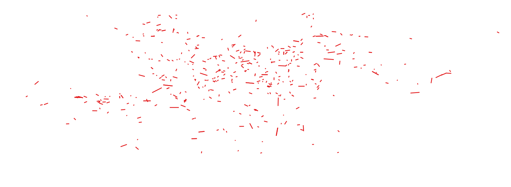
###Error distances between Wheelmap and Foursquare
Using the Foursquare venue and Wheelmap point, it is possible to see how much difference there is in where features are located. It also highlights the problem of features having the same name but not being the same real worl object. Entering the following code into the QGIS python console Plugins->Python Console adds a line layer to the map where each line links foursquare venues with wheelmap POIs with the same name. Depending on the layers you are working with, you will need to update the if lyr.name() == "wheelmap_helsinki": and if lyr.name() == "foursquare_venues_helsinki": accordingly. Note that this script may take some time to run, and if at the end the command for addMaplayer(vl) is visible in the bottom text box, you need to click in the text area and press the Enter key.
layers = iface.legendInterface().layers()
fsl = None
wml = None
for lyr in layers:
	if lyr.name() == "wheelmap_helsinki":
		wml = lyr
	if lyr.name() == "foursquare_venues_helsinki":
		fsl = lyr

vl = QgsVectorLayer('LineString?crs=epsg:4326', 'Linked features', "memory")
vp = vl.dataProvider()
vl.startEditing()
count = 0

for fsf in fsl.getFeatures():
	count = count+1
	for wmf in wml.getFeatures():
		if wmf["name"] == fsf["name"]:
			feat = QgsFeature(vl.pendingFields())
			feat.setGeometry(QgsGeometry.fromPolyline([fsf.geometry().asPoint(),wmf.geometry().asPoint()]))
			(res, outFeats) = vp.addFeatures([feat])
			break


	print str(count)

vl.commitChanges()
QgsMapLayerRegistry.instance().addMapLayer(vl)
As can be seen from running this code, a number of features may be linked even though they are on the other side of the city. Though this is important information, it obscure the information relating to slight differences in position. For now, we want to hide the lines that are over a specified length. To do this, we first need to calculate the length of the lines. First, right click on the new line layer and select Open attribute table. Next click on the field calculator button (the last one that looks like an abacus). Within this window, enter the name length under Output field name and select Decimal number (real) from the Output field type drop down. In the text box below the maths operators, enter $length to tell the calculator to fill this field with the length of the line. Click on OK and then close the attribute table. If you are asked to save any edits, choose the option that saves them. If you notice that most of the fields contain the text NULL, this is most likely because you had a line selected in the map interface and so the calculation was only applied to that feature. To add values to the other features, make sure that no features are selected (click on the button with a yellow box next to a no-entry symbol) and then repeat the field calculator process, but rather then adding an output field name, check the Update existing field box and select the length field from the drop down box below.
To filter out the long lines, right click on the line layer and select Filter.... This opens a window where you can apply rules similarly to the rule-based styling described above. If the Filter... option is disabled, you may need to first turn off editing (click on the pencil button in the editing toolbar). In the Provider specific filter expression text area, enter the text "length" <= 200 which tells the system to only show lines that have a length of less than 200m. Click OK to apply the filter, and then change the styling of the lines (Double click the layer in the Layers Panel, followed by the Style tab).
From the basic vector statistics for these lines that are less than 200m in length, we find that the average length is 39m.

