| theme | _class | paginate | backgroundColor | marp |
|---|---|---|---|---|
gaia |
lead |
true |
true |

第3讲: 深度学习基础 II
-
深度学习模型三要素
- 静: 模型结构、模型参数
- 动: 模型训练过程 (优化目标, 优化算法, ...)
- 学习素材: 数据(集)
-
“搞模型如同炒菜,食材、大厨、锅,缺一不可”
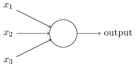
- 模型结构二要素: 结构定义, forward方法
- 结构定义:
class LeNet(nn.Module):
    def __init__(self):
        super().__init__()
        self.conv1 = nn.Conv2d(1, 6, 5)
        self.conv2 = nn.Conv2d(6, 16, 5)
        self.fc1 = nn.Linear(16*4*4, 120)
        self.fc2 = nn.Linear(120, 84)
self.fc3 = nn.Linear(84, 10)forward方法
def forward(self, x):
        x = nn.functional.relu(self.conv1(x))
        x = nn.functional.max_pool2d(x, 2, 2)
        x = nn.functional.relu(self.conv2(x))
        x = nn.functional.max_pool2d(x, 2, 2)
        x = x.view(-1, 16*4*4)
        x = nn.functional.relu(self.fc1(x))
        x = nn.functional.relu(self.fc2(x))
        x = self.fc3(x)
return x- 模型参数=$\sum$模型每层的参数
闪回模型的层
nn.Linear(input, output)- nn.Linear
- 参数: weight, bias
- 尺寸(shape): weight: (output, input), bias: (output)

linear = nn.Linear(5,3)
print(linear.weight.shape, linear.bias.shape)-
torch.matmal, @
-
torch.add, +
-
移步vscode,试一试,shape那些事,以及Tensor Broadcasting
试试这段代码
a = torch.randn(2, 2, 4)
print(a)
b = 20
a = a + b
print(a)

c = torch.randn(2,4)
a = a + c
print(c)
print(a)并行运算在深度学习时代非常重要
- N个样本,每个样本的shape (2, 4), 模型参数(2, 4)
- 一个batch的输入通常的shape (2, 2, 4)
- 如何为这个batch批量执行每个样本和模型参数的计算?
- 比如:
- Tensor 1 (2, 2, 4) * Tensor 2 (2, 4)
- Tensor 1 (2, 2, 4) @ Tensor 2 (4, 2)
- 比如:
- Each tensor must have at least one dimension - no empty tensors.
- Comparing the dimension sizes of the two tensors, going from last to first:
- Each dimension must be equal, or
- One of the dimensions must be of size 1, or
- The dimension does not exist in one of the tensors
来源: Introduction to PyTorch Tensors
-
nn.functional
-
激活函数(引入非线性)
- relu, sigmoid
-
池化
- average pooling, max pooling
- 1d, 2d, ...
- average pooling, max pooling
- 通过引入非线性函数(nonlinear function)可增加模型非线性的能力,在模型中中,也称之为激活函数
- 线性层:
$x=f(x)=xW^\top+b$ - 激活:
$x=activation(x)$
- 线性层:
- activation类型
- ReLU, Sigmoid, SwiGLU, ...


池化: “粗暴的”降维方法

池化: “粗暴的”降维方法

以分类问题举例
- 对于多分类问题而言,假设$\textbf{z}$是模型最终的原始输出,是非归一化(unnormalized)的表示,则用softmax函数赋予所有$z_i$概率含义
$\text{softmax}(\textbf{z})_i=\frac{\exp(z_i)}{\sum_j\exp(z_j)}$ - 其中,$\exp(x)=e^x$


- 构建模型的推理(inference)过程:计算图
def forward(self, x):
        x = nn.functional.relu(self.conv1(x))
        x = nn.functional.max_pool2d(x, 2, 2)
        x = nn.functional.relu(self.conv2(x))
        x = nn.functional.max_pool2d(x, 2, 2)
        x = x.view(-1, 16*4*4)
        x = nn.functional.relu(self.fc1(x))
        x = nn.functional.relu(self.fc2(x))
        x = self.fc3(x)
return xx = torch.ones(5) # input tensor
y = torch.zeros(3) # expected output
w = torch.randn(5, 3, requires_grad=True)
b = torch.randn(3, requires_grad=True)
z = torch.matmul(x, w)+b
loss = torch.nn.functional.binary_cross_entropy_with_logits(z, y)

- 假设,构建模型$f$,其参数为$\theta$
- 目标: 设计一种可用来度量基于$\theta$的模型预测结果和真实结果差距的度量,差距越小,模型越接近需估计的函数$f^*$
$J(\theta)=\frac{1}{n}\sum_{x\in \mathcal{X}}(f^*(x)-f(x;\theta))^2$
- 学习方法:梯度下降,寻找合适的$\theta$ (被称之训练模型)

- 目标:
$J(\theta)=\frac{1}{n}\sum_{x\in \mathcal{X}}(y-f(x;\theta))^2$
- 猜个$\theta$, 根据输入$x$,计算$\hat{y}=f(x;\theta)$
- 评估误差:
$y$ 和$\hat{y}$的误差(loss) - 根据误差,更新$\theta$:
$\theta=\theta -\lambda\cdot\Delta\theta$
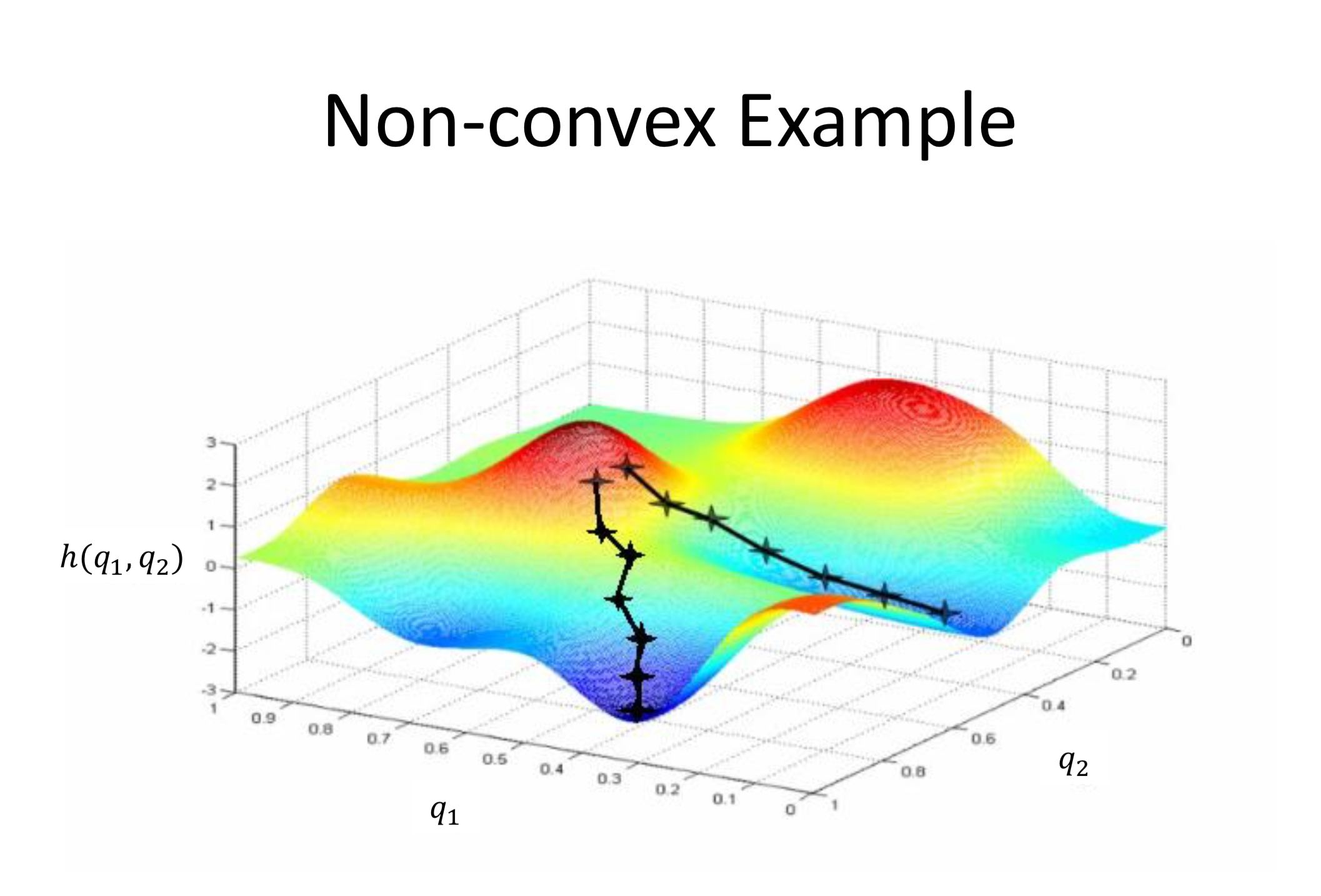
优化目标:
梯度下降法 (Gradient descent): 求偏导
-
$f^*(x)$ 通常以真值(groundtruth)体现,因此$\frac{\partial}{\partial \theta}J(\theta)$重点关注$f(x;\theta)$-
$f(x)=xW^\top+b$ -->$\frac{\partial}{\partial \theta}f(x)=\frac{\partial}{\partial \theta}(xW^\top+b)$ - 通常深度学习模型$f(x)$为复合函数,需利用链式法则求偏导
-
-
核心算法: 反向传播(backpropagation)
- 核心步骤: 针对优化目标$J(\theta)$求其偏导数(partial derivative)
-
假设深度学习模型为$f(x)=xW^\top+b$的复合函数
$y=f_3(f_2(f_1(x)))$
-
优化目标$J(\theta)$的偏导$\frac{\partial}{\partial \theta}J$的核心为$\frac{\partial}{\partial \theta}y=\frac{\partial}{\partial \theta}f_3(f_2(f_1(x)))$
-
链式法则展开:
$\frac{\partial J}{\partial \theta_{f_1}} = \frac{\partial J}{\partial y}\cdot \frac{\partial y}{\partial f_3}\cdot \frac{\partial f_3}{\partial f_2}\cdot \frac{\partial f_2}{\partial f_1} \cdot \frac{\partial f_1}{\partial \theta_{f_1}}$
-
偏导的构建
- 传统手工实现 v.s. autograd
-
“古代”手工实现
- forward: 代码实现$f(x)$
- backward: 手推偏导公式$\frac{\partial}{\partial \theta}f(x)$,照着公式进行代码实现
-
autograd
- forward: 基于forward实现构建计算图
- backward: 基于计算图实现自动微分(automatic differentiation)
参考阅读
目标:
- 猜个$\theta$, 根据输入$x$,计算$\hat{y}=f(x;\theta)$ -> 模型forward过程
- 评估误差:
$y$ 和$\hat{y}$的误差(loss) -> 选择loss function,并计算 - 根据误差,更新$\theta$:
$\theta=\theta -\lambda\cdot\Delta\theta$ -> 优化器更新模型参数
定义损失函数(loss),以及优化器(优化算法)
ce_loss = nn.CrossEntropyLoss()
optimizer = torch.optim.SGD(model.parameters(), lr=1e-3)-
常见损失函数,可在torch.nn中调用
- nn.CrossEntropyLoss, nn.L1Loss, nn.MSELoss, nn.NLLLoss, nn.KLDivLoss, nn.BCELoss, ...
-
常见优化算法,可在torch.optim中调用
- optim.SGD, optim.Adam, optim.AdamW, optim.LBFGS, ...
def train(dataloader, model, loss_fn, optimizer):
    size = len(dataloader.dataset)
    model.train()
    for batch, (X, y) in enumerate(dataloader):
        pred = model(X)
        l = loss_fn(pred, y)
        optimizer.zero_grad()
        l.backward()
        optimizer.step()
        if batch % 100 == 0:
            loss, current = l.item(), batch * len(X)
            print(f"loss: {loss:>7f}  [{current:>5d}/{size:>5d}]")
def test(dataloader, model, loss_fn):
    size = len(dataloader.dataset)
    num_batches = len(dataloader)
    model.eval()
    test_loss, correct = 0, 0
    with torch.no_grad():
        for X, y in dataloader:
            pred = model(X)
            test_loss += loss_fn(pred, y).item()
            correct += (pred.argmax(1) == y).type(torch.float).sum().item()
    test_loss /= num_batches
    correct /= size
    print(f"Test Error: \n Accuracy: {(100*correct):>0.1f}%, Avg loss: {test_loss:>8f} \n")
    return correct